Graphs

Introduction

PyX can be used for data and function plotting. At present x-y-graphs and x-y-z-graphs are supported only. However, the component architecture of the graph system described in section Component architecture allows for additional graph geometries while reusing most of the existing components.

Creating a graph splits into two basic steps. First you have to create a graph instance. The most simple form would look like:

from pyx import *
g = graph.graphxy(width=8)

The graph instance g created in this example can then be used to actually plot something into the graph. Suppose you have some data in a file graph.dat you want to plot. The content of the file could look like:

1   2
2   3
3   8
4  13
5  18
6  21

To plot these data into the graph g you must perform:

g.plot(graph.data.file("graph.dat", x=1, y=2))

The method plot() takes the data to be plotted and optionally a list of graph styles to be used to plot the data. When no styles are provided, a default style defined by the data instance is used. For data read from a file by an instance of graph.data.file, the default are symbols. When instantiating graph.data.file, you not only specify the file name, but also a mapping from columns to axis names and other information the styles might make use of (e.g. data for error bars to be used by the errorbar style).

While the graph is already created by that, we still need to perform a write of the result into a file. Since the graph instance is a canvas, we can just call its writeEPSfile() method.

g.writeEPSfile("graph")

The result graph.eps is shown in figure A minimalistic plot for the data from file graph.dat..

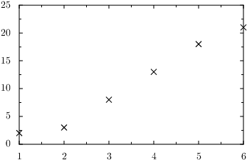
A minimalistic plot for the data from file graph.dat.

Instead of plotting data from a file, other data source are available as well. For example function data is created and placed into plot() by the following line:

g.plot(graph.data.function("y(x)=x**2"))

You can plot different data in a single graph by calling plot() several times before writing the output to a file. Note that a calling plot() will fail once a graph was forced to “finish” itself. This happens automatically, when the graph is written to a file. Thus it is not an option to call plot() after writing the output. The topic of the finalization of a graph is addressed in more detail in section graph.graph. As you can see in figure Plotting data from a file together with a function., a function is plotted as a line by default.

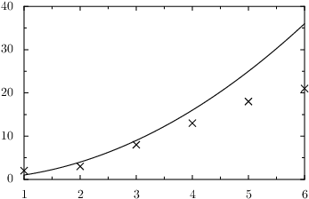
Plotting data from a file together with a function.

While the axes ranges got adjusted automatically in the previous example, they might be fixed by keyword options in axes constructors. Plotting only a function will need such a setting at least in the variable coordinate. The following code also shows how to set a logathmic axis in y-direction:

from pyx import *
g = graph.graphxy(width=8, x=graph.axis.linear(min=-5, max=5),
                           y=graph.axis.logarithmic())
g.plot(graph.data.function("y(x)=exp(x)"))
g.writePDFfile()

The result is shown in figure Plotting a function for a given axis range and use a logarithmic y-axis..

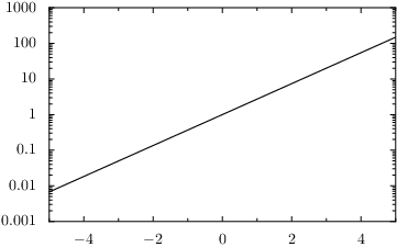
Plotting a function for a given axis range and use a logarithmic y-axis.

Component architecture

Creating a graph involves a variety of tasks, which thus can be separated into components without significant additional costs. This structure manifests itself also in the PyX source, where there are different modules for the different tasks. They interact by some well-defined interfaces. They certainly have to be completed and stabilized in their details, but the basic structure came up in the continuous development quite clearly. The basic parts of a graph are:

graph

Defines the geometry of the graph by means of graph coordinates with range [0:1]. Keeps lists of plotted data, axes etc.

data

Produces or prepares data to be plotted in graphs.

style

Performs the plotting of the data into the graph. It gets data, converts them via the axes into graph coordinates and uses the graph to finally plot the data with respect to the graph geometry methods.

key

Responsible for the graph keys.

axis

Creates axes for the graph, which take care of the mapping from data values to graph coordinates. Because axes are also responsible for creating ticks and labels, showing up in the graph themselves and other things, this task is split into several independent subtasks. Axes are discussed separately in chapter axis.

Module graph.graph: Graph geometry

The classes graphxy and graphxyz are part of the module graph.graph. However, there are shortcuts to access the classes via graph.graphxy and graph.graphxyz, respectively.

class graph.graph.graphxy(xpos=0, ypos=0, width=None, height=None, ratio=goldenmean, key=None, backgroundattrs=None, axesdist=0.8 * unit.v_cm, xaxisat=None, yaxisat=None, **axes)

This class provides an x-y-graph. A graph instance is also a fully functional canvas.

The position of the graph on its own canvas is specified by xpos and ypos. The size of the graph is specified by width, height, and ratio. These parameters define the size of the graph area not taking into account the additional space needed for the axes. Note that you have to specify at least width or height. ratio will be used as the ratio between width and height when only one of these is provided.

key can be set to a graph.key.key instance to create an automatic graph key. None omits the graph key.

backgroundattrs is a list of attributes for drawing the background of the graph. Allowed are decorators, strokestyles, and fillstyles. None disables background drawing.

axisdist is the distance between axes drawn at the same side of a graph.

xaxisat and yaxisat specify a value at the y and x axis, where the corresponding axis should be moved to. It’s a shortcut for corresonding calls of axisatv() described below. Moving an axis by xaxisat or yaxisat disables the automatic creation of a linked axis at the opposite side of the graph.

**axes receives axes instances. Allowed keywords (axes names) are x, x2, x3, etc. and y, y2, y3, etc. When not providing an x or y axis, linear axes instances will be used automatically. When not providing a x2 or y2 axis, linked axes to the x and y axes are created automatically and vice versa. As an exception, a linked axis is not created automatically when the axis is placed at a specific position by xaxisat or yaxisat. You can disable the automatic creation of axes by setting the linked axes to None. The even numbered axes are plotted at the top (x axes) and right (y axes) while the others are plotted at the bottom (x axes) and left (y axes) in ascending order each.

Some instance attributes might be useful for outside read-access. Those are:

graphxy.axes

A dictionary mapping axes names to the anchoredaxis instances.

To actually plot something into the graph, the following instance method plot() is provided:

graphxy.plot(data, styles=None)

Adds data to the list of data to be plotted. Sets styles to be used for plotting the data. When styles is None, the default styles for the data as provided by data is used.

data should be an instance of any of the data described in section graph.data.

When the same combination of styles (i.e. the same references) are used several times within the same graph instance, the styles are kindly asked by the graph to iterate their appearance. Its up to the styles how this is performed.

Instead of calling the plot method several times with different data but the same style, you can use a list (or something iterateable) for data.

While a graph instance only collects data initially, at a certain point it must create the whole plot. Once this is done, further calls of plot() will fail. Usually you do not need to take care about the finalization of the graph, because it happens automatically once you write the plot into a file. However, sometimes position methods (described below) are nice to be accessible. For that, at least the layout of the graph must have been finished. However, the drawing order is based on canvas layers and thus the order in which the do()-methods are called will not alter the output. Multiple calls to any of the do()-methods have no effect (only the first call counts). The orginal order in which the do()-methods are called is:

graphxy.dolayout()

Fixes the layout of the graph. As part of this work, the ranges of the axes are fitted to the data when the axes ranges are allowed to adjust themselves to the data ranges. The other do()-methods ensure, that this method is always called first.

graphxy.dobackground()

Draws the background.

graphxy.doaxes()

Inserts the axes.

graphxy.doplotitem(plotitem)

Plots the plotitem as returned by the graphs plot method.

graphxy.doplot()

Plots all (remaining) plotitems.

graphxy.dokeyitem()

Inserts a plotitem in the graph key as returned by the graphs plot method.

graphxy.dokey()

Inserts the graph key.

graphxy.finish()

Finishes the graph by calling all pending do()-methods. This is done automatically, when the output is created.

The graph provides some methods to access its geometry:

graphxy.pos(x, y, xaxis=None, yaxis=None)

Returns the given point at x and y as a tuple (xpos, ypos) at the graph canvas. x and y are anchoredaxis instances for the two axes xaxis and yaxis. When xaxis or yaxis are None, the axes with names x and y are used. This method fails if called before dolayout().

graphxy.vpos(vx, vy)

Returns the given point at vx and vy as a tuple (xpos, ypos) at the graph canvas. vx and vy are graph coordinates with range [0:1].

graphxy.vgeodesic(vx1, vy1, vx2, vy2)

Returns the geodesic between points vx1, vy1 and vx2, vy2 as a path. All parameters are in graph coordinates with range [0:1]. For graphxy this is a straight line.

graphxy.vgeodesic_el(vx1, vy1, vx2, vy2)

Like vgeodesic() but this method returns the path element to connect the two points.

Further geometry information is available by the axes instance variable, with is a dictionary mapping axis names to anchoredaxis instances. Shortcuts to the anchoredaxis positioner methods for the x- and y-axis become available after dolayout() as graphxy methods Xbasepath, Xvbasepath, Xgridpath, Xvgridpath, Xtickpoint, Xvtickpoint, Xtickdirection, and Xvtickdirection where the prefix X stands for x and y.

graphxy.axistrafo(axis, t)

This method can be used to apply a transformation t to an anchoredaxis instance axis to modify the axis position and the like. This method fails when called on a not yet finished axis, i.e. it should be used after dolayout().

graphxy.axisatv(axis, v)

This method calls axistrafo() with a transformation to move the axis axis to a graph position v (in graph coordinates).

The class graphxyz is very similar to the graphxy class, except for its additional dimension. In the following documentation only the differences to the graphxy class are described.

class graph.graph.graphxyz(xpos=0, ypos=0, size=None, xscale=1, yscale=1, zscale=1 / goldenmean, xy12axesat=None, xy12axesatname='z', projector=central(10, -30, 30), key=None, **axes)

This class provides an x-y-z-graph.

The position of the graph on its own canvas is specified by xpos and ypos. The size of the graph is specified by size and the length factors xscale, yscale, and zscale. The final size of the graph depends on the projector projector, which is called with x, y, and z values up to xscale, yscale, and zscale respectively and scaling the result by size. For a parallel projector changing size is thus identical to changing xscale, yscale, and zscale by the same factor. For the central projector the projectors internal distance would also need to be changed by this factor. Thus size changes the size of the whole graph without changing the projection.

xy12axesat moves the xy-plane of the axes x, x2, y, y2 to the given value at the axis xy12axesatname.

projector defines the conversion of 3d coordinates to 2d coordinates. It can be an instance of central or parallel described below.

**axes receives axes instances as for graphxy. The graphxyz allows for 4 axes per graph dimension x, x2, x3, x4, y, y2, y3, y4, z, z2, z3, and z4. The x-y-plane is the horizontal plane at the bottom and the x, x2, y, and y2 axes are placed at the boundary of this plane with x and y always being in front. x3, x4, y3, and y4 are handled similar, but for the top plane of the graph. The z axis is placed at the origin of the x and y dimension, whereas z2 is placed at the final point of the x dimension, z3 at the final point of the y dimension and z4 at the final point of the x and y dimension together.

graphxyz.central

The central attribute of the graphxyz is the central class. See the class description below.

graphxyz.parallel

The parallel attribute of the graphxyz is the parallel class. See the class description below.

Regarding the 3d to 2d transformation the methods pos(), vpos(), vgeodesic(), and vgeodesic_el() are available as for class graphxy and just take an additional argument for the dimension. Note that a similar transformation method (3d to 2d) is available as part of the projector as well already, but only the graph acknowledges its size, the scaling and the internal tranformation of the graph coordinates to the scaled coordinates. As the projector also implements a zindex() and a angle() method, those are also available at the graph level in the graph coordinate variant (i.e. having an additional v in its name and using values from 0 to 1 per dimension).

graphxyz.vzindex(vx, vy, vz)

The depths of the point defined by vx, vy, and vz scaled to a range [-1:1] where 1 is closest to the viewer. All arguments passed to the method are in graph coordinates with range [0:1].

graphxyz.vangle(vx1, vy1, vz1, vx2, vy2, vz2, vx3, vy3, vz3)

The cosine of the angle of the view ray thru point (vx1, vy1, vz1) and the plane defined by the points (vx1, vy1, vz1), (vx2, vy2, vz2), and (vx3, vy3, vz3). All arguments passed to the method are in graph coordinates with range [0:1].

There are two projector classes central and parallel:

class graph.graph.central(distance, phi, theta, anglefactor=math.pi / 180)

Instances of this class implement a central projection for the given parameters.

distance is the distance of the viewer from the origin. Note that the graphxyz class uses the range -xscale to xscale, -yscale to yscale, and -zscale to zscale for the coordinates x, y, and z. As those scales are of the order of one (by default), the distance should be of the order of 10 to give nice results. Smaller distances increase the central projection character while for huge distances the central projection becomes identical to the parallel projection.

phi is the angle of the viewer in the x-y-plane and theta is the angle of the viewer to the x-y-plane. The standard notation for spheric coordinates are used. The angles are multiplied by anglefactor which is initialized to do a degree in radiant transformation such that you can specify phi and theta in degree while the internal computation is always done in radiants.

class graph.graph.parallel(phi, theta, anglefactor=math.pi / 180)

Instances of this class implement a parallel projection for the given parameters. There is no distance for that transformation (compared to the central projection). All other parameters are identical to the central class.

Module graph.data: Graph data

The following classes provide data for the plot() method of a graph. The classes are implemented in graph.data.

class graph.data.file(filename, commentpattern=defaultcommentpattern, columnpattern=defaultcolumnpattern, stringpattern=defaultstringpattern, skiphead=0, skiptail=0, every=1, title=notitle, context={}, copy=1, replacedollar=1, columncallback='__column__', **columns)

This class reads data from a file and makes them available to the graph system. filename is the name of the file to be read. The data should be organized in columns.

The arguments commentpattern, columnpattern, and stringpattern are responsible for identifying the data in each line of the file. Lines matching commentpattern are ignored except for the column name search of the last non- empty comment line before the data. By default a line starting with one of the characters '#', '%', or '!' as well as an empty line is treated as a comment.

A non-comment line is analysed by repeatedly matching stringpattern and, whenever the stringpattern does not match, by columnpattern. When the stringpattern matches, the result is taken as the value for the next column without further transformations. When columnpattern matches, it is tried to convert the result to a float. When this fails the result is taken as a string as well. By default, you can write strings with spaces surrounded by '"' immediately surrounded by spaces or begin/end of line in the data file. Otherwise '"' is not taken to be special.

skiphead and skiptail are numbers of data lines to be ignored at the beginning and end of the file while every selects only every every line from the data.

title is the title of the data to be used in the graph key. A default title is constructed out of filename and **columns. You may set title to None to disable the title.

Finally, columns define columns out of the existing columns from the file by a column number or a mathematical expression (see below). When copy is set the names of the columns in the file (file column names) and the freshly created columns having the names of the dictionary key (data column names) are passed as data to the graph styles. The data columns may hide file columns when names are equal. For unset copy the file columns are not available to the graph styles.

File column names occur when the data file contains a comment line immediately in front of the data (except for empty or empty comment lines). This line will be parsed skipping the matched comment identifier as if the line would be regular data, but it will not be converted to floats even if it would be possible to convert the items. The result is taken as file column names, i.e. a string representation for the columns in the file.

The values of **columns can refer to column numbers in the file starting at 1. The column 0 is also available and contains the line number starting from 1 not counting comment lines, but lines skipped by skiphead, skiptail, and every. Furthermore values of **columns can be strings: file column names or complex mathematical expressions. To refer to columns within mathematical expressions you can also use file column names when they are valid variable identifiers. Equal named items in context will then be hidden. Alternatively columns can be access by the syntax $<number> when replacedollar is set. They will be translated into function calls to columncallback, which is a function to access column data by index or name.

context allows for accessing external variables and functions when evaluating mathematical expressions for columns. Additionally to the identifiers in context, the file column names, the columncallback function and the functions shown in the table “builtins in math expressions” at the end of the section are available.

Example:

graph.data.file("test.dat", a=1, b="B", c="2*B+$3")

with test.dat looking like:

# A   B C
1.234 1 2
5.678 3 4

The columns with name "a", "b", "c" will become "[1.234, 5.678]", "[1.0, 3.0]", and "[4.0, 10.0]", respectively. The columns "A", "B", "C" will be available as well, since copy is enabled by default.

When creating several data instances accessing the same file, the file is read only once. There is an inherent caching of the file contents.

For the sake of completeness we list the default patterns:

file.defaultcommentpattern

re.compile(r"(#+|!+|%+)\s*")

file.defaultcolumnpattern

re.compile(r"\"(.*?)\"(\s+|$)")

file.defaultstringpattern

re.compile(r"(.*?)(\s+|$)")

class graph.data.function(expression, title=notitle, min=None, max=None, points=100, context={})

This class creates graph data from a function. expression is the mathematical expression of the function. It must also contain the result variable name including the variable the function depends on by assignment. A typical example looks like "y(x)=sin(x)".

title is the title of the data to be used in the graph key. By default expression is used. You may set title to None to disable the title.

min and max give the range of the variable. If not set, the range spans the whole axis range. The axis range might be set explicitly or implicitly by ranges of other data. points is the number of points for which the function is calculated. The points are choosen linearly in terms of graph coordinates.

context allows for accessing external variables and functions. Additionally to the identifiers in context, the variable name and the functions shown in the table “builtins in math expressions” at the end of the section are available.

class graph.data.paramfunction(varname, min, max, expression, title=notitle, points=100, context={})

This class creates graph data from a parametric function. varname is the parameter of the function. min and max give the range for that variable. points is the number of points for which the function is calculated. The points are choosen lineary in terms of the parameter.

expression is the mathematical expression for the parametric function. It contains an assignment of a tuple of functions to a tuple of variables. A typical example looks like "x, y = cos(k), sin(k)".

title is the title of the data to be used in the graph key. By default expression is used. You may set title to None to disable the title.

context allows for accessing external variables and functions. Additionally to the identifiers in context, varname and the functions shown in the table “builtins in math expressions” at the end of the section are available.

class graph.data.values(title='user provided values', **columns)

This class creates graph data from externally provided data. Each column is a list of values to be used for that column.

title is the title of the data to be used in the graph key.

class graph.data.points(data, title='user provided points', addlinenumbers=1, **columns)

This class creates graph data from externally provided data. data is a list of lines, where each line is a list of data values for the columns.

title is the title of the data to be used in the graph key.

The keywords of **columns become the data column names. The values are the column numbers starting from one, when addlinenumbers is turned on (the zeroth column is added to contain a line number in that case), while the column numbers starts from zero, when addlinenumbers is switched off.

class graph.data.data(data, title=notitle, context=, copy=1, replacedollar=1, columncallback="__column__", **columns)

This class provides graph data out of other graph data. data is the source of the data. All other parameters work like the equally called parameters in graph.data.file. Indeed, the latter is built on top of this class by reading the file and caching its contents in a graph.data.list instance.

class graph.data.conffile(filename, title=notitle, context=, copy=1, replacedollar=1, columncallback="__column__", **columns)

This class reads data from a config file with the file name filename. The format of a config file is described within the documentation of the ConfigParser module of the Python Standard Library.

Each section of the config file becomes a data line. The options in a section are the columns. The name of the options will be used as file column names. All other parameters work as in graph.data.file and graph.data.data since they all use the same code.

class graph.data.cbdfile(filename, minrank=None, maxrank=None, title=notitle, context=, copy=1, replacedollar=1, columncallback="__column__", **columns)

This is an experimental class to read map data from cbd-files. See http://sepwww.stanford.edu/ftp/World_Map/ for some world-map data.

The builtins in math expressions are listed in the following table:

name	value
neg	lambda x: -x
abs	lambda x: x < 0 and -x or x
sgn	lambda x: x < 0 and -1 or 1
sqrt	math.sqrt
exp	math.exp
log	math.log
sin	math.sin
cos	math.cos
tan	math.tan
asin	math.asin
acos	math.acos
atan	math.atan
sind	lambda x: math.sin(math.pi/180*x)
cosd	lambda x: math.cos(math.pi/180*x)
tand	lambda x: math.tan(math.pi/180*x)
asind	lambda x: 180/math.pi*math.asin(x)
acosd	lambda x: 180/math.pi*math.acos(x)
atand	lambda x: 180/math.pi*math.atan(x)
norm	lambda x, y: math.hypot(x, y)
splitatvalue	see the splitatvalue description below
pi	math.pi
e	math.e

math refers to Pythons math module. The splitatvalue function is defined as:

graph.data.splitatvalue(value, *splitpoints)

This method returns a tuple (section, value). The section is calculated by comparing value with the values of splitpoints. If splitpoints contains only a single item, section is 0 when value is lower or equal this item and 1 else. For multiple splitpoints, section is 0 when its lower or equal the first item, None when its bigger than the first item but lower or equal the second item, 1 when its even bigger the second item, but lower or equal the third item. It continues to alter between None and 2, 3, etc.

Module graph.style: Graph styles

Please note that we are talking about graph styles here. Those are responsible for plotting symbols, lines, bars and whatever else into a graph. Do not mix it up with path styles like the line width, the line style (solid, dashed, dotted etc.) and others.

The following classes provide styles to be used at the plot() method of a graph. The plot method accepts a list of styles. By that you can combine several styles at the very same time.

Some of the styles below are hidden styles. Those do not create any output, but they perform internal data handling and thus help on modularization of the styles. Usually, a visible style will depend on data provided by one or more hidden styles but most of the time it is not necessary to specify the hidden styles manually. The hidden styles register themself to be the default for providing certain internal data.

class graph.style.pos(usenames={}, epsilon=1e-10)

This class is a hidden style providing a position in the graph. It needs a data column for each graph dimension. For that the column names need to be equal to an axis name, or a name translation from axis names to column names need to be given by usenames. Data points are considered to be out of graph when their position in graph coordinates exceeds the range [0:1] by more than epsilon.

class graph.style.range(usenames={}, epsilon=1e-10)

This class is a hidden style providing an errorbar range. It needs data column names constructed out of a axis name X for each dimension errorbar data should be provided as follows:

data name	description
Xmin	minimal value
Xmax	maximal value
dX	minimal and maximal delta
dXmin	minimal delta
dXmax	maximal delta

When delta data are provided the style will also read column data for the axis name X itself. usenames allows to insert a translation dictionary from axis names to the identifiers X.

epsilon is a comparison precision when checking for invalid errorbar ranges.

class graph.style.symbol(symbol=changecross, size=0.2 * unit.v_cm, symbolattrs=[])

This class is a style for plotting symbols in a graph. symbol refers to a (changeable) symbol function with the prototype symbol(c, x_pt, y_pt, size_pt, attrs) and draws the symbol into the canvas c at the position (x_pt, y_pt) with size size_pt and attributes attrs. Some predefined symbols are available in member variables listed below. The symbol is drawn at size size using symbolattrs. symbolattrs is merged with defaultsymbolattrs which is a list containing the decorator deco.stroked. An instance of symbol is the default style for all graph data classes described in section graph.data except for function and paramfunction.

The class symbol provides some symbol functions as member variables, namely:

symbol.cross

A cross. Should be used for stroking only.

symbol.plus

A plus. Should be used for stroking only.

symbol.square

A square. Might be stroked or filled or both.

symbol.triangle

A triangle. Might be stroked or filled or both.

symbol.circle

A circle. Might be stroked or filled or both.

symbol.diamond

A diamond. Might be stroked or filled or both.

symbol provides some changeable symbol functions as member variables, namely:

symbol.changecross

attr.changelist([cross, plus, square, triangle, circle, diamond])

symbol.changeplus

attr.changelist([plus, square, triangle, circle, diamond, cross])

symbol.changesquare

attr.changelist([square, triangle, circle, diamond, cross, plus])

symbol.changetriangle

attr.changelist([triangle, circle, diamond, cross, plus, square])

symbol.changecircle

attr.changelist([circle, diamond, cross, plus, square, triangle])

symbol.changediamond

attr.changelist([diamond, cross, plus, square, triangle, circle])

symbol.changesquaretwice

attr.changelist([square, square, triangle, triangle, circle, circle, diamond, diamond])

symbol.changetriangletwice

attr.changelist([triangle, triangle, circle, circle, diamond, diamond, square, square])

symbol.changecircletwice

attr.changelist([circle, circle, diamond, diamond, square, square, triangle, triangle])

symbol.changediamondtwice

attr.changelist([diamond, diamond, square, square, triangle, triangle, circle, circle])

The class symbol provides two changeable decorators for alternated filling and stroking. Those are especially useful in combination with the change()-twice()-symbol methods above. They are:

symbol.changestrokedfilled

attr.changelist([deco.stroked, deco.filled])

symbol.changefilledstroked

attr.changelist([deco.filled, deco.stroked])

class graph.style.line(lineattrs=[], epsilon=1e-10)

This class is a style to stroke lines in a graph. lineattrs is merged with defaultlineattrs which is a list containing the member variable changelinestyle as described below. An instance of line is the default style of the graph data classes function and paramfunction described in section graph.data. epsilon is a precision in graph coordinates for line clipping.

The class line provides a changeable line style. Its definition is:

line.changelinestyle

attr.changelist([style.linestyle.solid, style.linestyle.dashed, style.linestyle.dotted, style.linestyle.dashdotted])

class graph.style.impulses(lineattrs=[], fromvalue=0, frompathattrs=[], valueaxisindex=1)

This class is a style to plot impulses. lineattrs is merged with defaultlineattrs which is a list containing the member variable changelinestyle of the line class. fromvalue is the baseline value of the impulses. When set to None, the impulses will start at the baseline. When fromvalue is set, frompathattrs are the stroke attributes used to show the impulses baseline path.

class graph.style.errorbar(size=0.1 * unit.v_cm, errorbarattrs=[], epsilon=1e-10)

This class is a style to stroke errorbars in a graph. size is the size of the caps of the errorbars and errorbarattrs are the stroke attributes. Errorbars and error caps are considered to be out of the graph when their position in graph coordinates exceeds the range [0:1] by more that epsilon. Out of graph caps are omitted and the errorbars are cut to the valid graph range.

class graph.style.text(textname='text', dxname=None, dyname=None, dxunit=0.3 * unit.v_cm, dyunit=0.3 * unit.v_cm, textdx=0 * unit.v_cm, textdy=0.3 * unit.v_cm, textattrs=[])

This class is a style to stroke text in a graph. The text to be written has to be provided in the data column named textname. textdx and textdy are the position of the text with respect to the position in the graph. Alternatively you can specify a dxname and a dyname and provide appropriate data in those columns to be taken in units of dxunit and dyunit to specify the position of the text for each point separately. textattrs are text attributes for the output of the text. Those attributes are merged with the default attributes textmodule.halign.center and textmodule.vshift.mathaxis.

class graph.style.arrow(linelength=0.25 * unit.v_cm, arrowsize=0.15 * unit.v_cm, lineattrs=[], arrowattrs=[], arrowpos=0.5, epsilon=1e-10, decorator=deco.earrow)

This class is a style to plot short lines with arrows into a two-dimensional graph to a given graph position. The arrow parameters are defined by two additional data columns named size and angle define the size and angle for each arrow. size is taken as a factor to arrowsize and linelength, the size of the arrow and the length of the line the arrow is plotted at. angle is the angle the arrow points to with respect to a horizontal line. The angle is taken in degrees and used in mathematically positive sense. lineattrs and arrowattrs are styles for the arrow line and arrow head, respectively. arrowpos defines the position of the arrow line with respect to the position at the graph. The default 0.5 means centered at the graph position, whereas 0 and 1 creates the arrows to start or end at the graph position, respectively. epsilon is used as a cutoff for short arrows in order to prevent numerical instabilities. decorator defines the decorator to be added to the line.

class graph.style.rect(colorname='color', gradient=color.gradient.Grey, coloraxis=None, keygraph=_autokeygraph)

This class is a style to plot colored rectangles into a two-dimensional graph. The size of the rectangles is taken from the data provided by the range style. The additional data column named colorname specifies the color of the rectangle defined by gradient. The translation of the data values to the gradient is done by the coloraxis, which is set to be a linear axis if not provided by coloraxis. A key graph, a graphx instance, is generated automatically to indicate the color scale if not provided by keygraph. If a keygraph is given, its x axis defines the color conversion and coloraxis is ignored.

class graph.style.histogram(lineattrs=[], steps=0, fromvalue=0, frompathattrs=[], fillable=0, rectkey=0, autohistogramaxisindex=0, autohistogrampointpos=0.5, epsilon=1e-10)

This class is a style to plot histograms. lineattrs is merged with defaultlineattrs which is [deco.stroked]. When steps is set, the histrogram is plotted as steps instead of the default being a boxed histogram. fromvalue is the baseline value of the histogram. When set to None, the histogram will start at the baseline. When fromvalue is set, frompathattrs are the stroke attributes used to show the histogram baseline path.

The fillable flag changes the stoke line of the histogram to make it fillable properly. This is important on non-steped histograms or on histograms, which hit the graph boundary. rectkey can be set to generate a rectanglar area instead of a line in the graph key.

In the most general case, a histogram is defined by a range specification (like for an errorbar) in one graph dimension (say, along the x-axis) and a value for the other graph dimension. This allows for the widths of the histogram boxes being variable. Often, however, all histogram bin ranges are equally sized, and instead of passing the range, the position of the bin along the x-axis fully specifies the histogram - assuming that there are at least two bins. This common case is supported via two parameters: autohistogramaxisindex, which defines the index of the independent histogram axis (in the case just described this would be 0 designating the x axis). autohistogrampointpos, defines the relative position of the center of the histogram bin: 0.5 means that the bin is centered at the values passed to the style, 0 (1) means that the bin is aligned at the right-(left-)hand side.

XXX describe, how to specify general histograms with varying bin widths

Positions of the histograms are considered to be out of graph when they exceed the graph coordinate range [0:1] by more than epsilon.

class graph.style.barpos(fromvalue=None, frompathattrs=[], epsilon=1e-10)

This class is a hidden style providing position information in a bar graph. Those graphs need to contain a specialized axis, namely a bar axis. The data column for this bar axis is named Xname where X is an axis name. In the other graph dimension the data column name must be equal to an axis name. To plot several bars in a single graph side by side, you need to have a nested bar axis and provide a tuple as data for nested bar axis.

The bars start at fromvalue when provided. The fromvalue is marked by a gridline stroked using frompathattrs. Thus this hidden style might actually create some output. The value of a bar axis is considered to be out of graph when its position in graph coordinates exceeds the range [0:1] by more than epsilon.

class graph.style.stackedbarpos(stackname, addontop=0, epsilon=1e-10)

This class is a hidden style providing position information in a bar graph by stacking a new bar on top of another bar. The value of the new bar is taken from the data column named stackname. When addontop is set, the values is taken relative to the previous top of the bar.

class graph.style.bar(barattrs=[], epsilon=1e-10, gradient=color.gradient.RedBlack)

This class draws bars in a bar graph. The bars are filled using barattrs. barattrs is merged with defaultbarattrs which is a list containing [color.gradient.Rainbow, deco.stroked([color.grey.black])].

The bar style has limited support for 3d graphs: Occlusion does not work properly on stacked bars or multiple dataset. epsilon is used in 3d to prevent numerical instabilities on bars without hight. When gradient is not None it is used to calculate a lighting coloring taking into account the angle between the view ray and the bar and the distance between viewer and bar. The precise conversion is defined in the lighting() method.

class graph.style.changebar(barattrs=[])

This style works like the bar style, but instead of the barattrs to be changed on subsequent data instances the barattrs are changed for each value within a single data instance. In the result the style can’t be applied to several data instances and does not support 3d. The style raises an error instead.

class graph.style.gridpos(index1=0, index2=1, gridlines1=1, gridlines2=1, gridattrs=[], epsilon=1e-10)

This class is a hidden style providing rectangular grid information out of graph positions for graph dimensions index1 and index2. Data points are considered to be out of graph when their position in graph coordinates exceeds the range [0:1] by more than epsilon. Data points are merged to a single graph coordinate value when their difference in graph coordinates is below epsilon.

class graph.style.grid(gridlines1=1, gridlines2=1, gridattrs=[], epsilon=1e-10)

Strokes a rectangular grid in the first grid direction, when gridlines1 is set and in the second grid direction, when gridlines2 is set. gridattrs is merged with defaultgridattrs which is a list containing the member variable changelinestyle of the line class. epsilon is a precision in graph coordinates for line clipping.

class graph.style.surface(gridlines1=0.05, gridlines2=0.05, gridcolor=None, backcolor=color.gray.black, **kwargs)

Draws a surface of a rectangular grid. Each rectangle is divided into 4 triangles.

If a gridcolor is set, the rectangular grid is marked by small stripes of the relative (compared to each rectangle) size of gridlines1 and gridlines2 for the first and second grid direction, respectively.

backcolor is used to fill triangles shown from the back. If backcolor is set to None, back sides are not drawn differently from the front sides.

The surface is encoded using a single mesh. While this is quite space efficient, it has the following implications:

• All colors must use the same color space.

• HSB colors are not allowed, whereas Gray, RGB, and CMYK are allowed. You can

  convert HSB colors into a different color space by means of rgbgradient and class:cmykgradient before passing it to the surface style.

• The grid itself is also constructed out of triangles. The grid is transformed

  along with the triangles thus looking quite different from a stroked grid (as done by the grid style).

• Occlusion is handled by proper painting order.

• Color changes are continuous (in the selected color space) for each triangle.

  Further arguments are identical to the graph.style.rect style. However, if no colorname column exists, the surface style falls back to a lighting coloring taking into account the angle between the view ray and the triangle and the distance between viewer and triangle. The precise conversion is defined in the lighting() method.

density(epsilon=1e-10, **kwargs):

Density plots can be created by the density style. It is similar to a surface plot in 2d, but it does not use a mesh, but a bitmap representation instead. Due to that difference, the file size is smaller and no color interpolation takes place. Furthermore the style can be used with equidistantly spaced data only (after conversion by the axis, so logarithmic raw data and such are possible using proper axes). Further arguments are identical to the graph.style.rect style.

Module graph.key: Graph keys

The following class provides a key, whose instances can be passed to the constructor keyword argument key of a graph. The class is implemented in graph.key.

class graph.key.key(dist=0.2 * unit.v_cm, pos='tr', hpos=None, vpos=None, hinside=1, vinside=1, hdist=0.6 * unit.v_cm, vdist=0.4 * unit.v_cm, symbolwidth=0.5 * unit.v_cm, symbolheight=0.25 * unit.v_cm, symbolspace=0.2 * unit.v_cm, textattrs=[], columns=1, columndist=0.5 * unit.v_cm, border=0.3 * unit.v_cm, keyattrs=None)

This class writes the title of the data in a plot together with a small illustration of the style. The style is responsible for its illustration.

dist is a visual length and a distance between the key entries. pos is the position of the key with respect to the graph. Allowed values are combinations of "t" (top), "m" (middle) and "b" (bottom) with "l" (left), "c" (center) and "r" (right). Alternatively, you may use hpos and vpos to specify the relative position using the range [0:1]. hdist and vdist are the distances from the specified corner of the graph. hinside and vinside are numbers to be set to 0 or 1 to define whether the key should be placed horizontally and vertically inside of the graph or not.

symbolwidth and symbolheight are passed to the style to control the size of the style illustration. symbolspace is the space between the illustration and the text. textattrs are attributes for the text creation. They are merged with [text.vshift.mathaxis].

columns is a number of columns of the graph key and columndist is the distance between those columns.

When keyattrs is set to contain some draw attributes, the graph key is enlarged by border and the key area is drawn using keyattrs.