PyX — Example: drawing2/ellipse.py

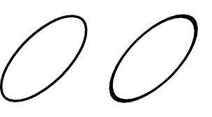
PyX does not directly provide a path corresponding to an ellipse. This example shows two ways how to draw an ellipse using affine transformations.

In order to create an ellipse, we best start from a unit circle centered around the point of origin of the coordinate system (here: circ). In variant 1, we tell PyX to apply a couple of affine transformations before stroking this circle on the canvas c. These affine transformations are contained in the trafo module. We first use trafo.scale to apply a non-uniform scaling, namely by a factor of 2 in x-direction and a factor of 0.9 in y-direction. Doing so, we define the two principle axes of the ellipse. In a next step, we rotate with trafo.rotate the ellipse by an angle of 45 degrees in the mathematical positive direction, i.e. counter-clockwise. Last, we shift the origin of the ellipse to the desired point by applying a trafo.translate operation.

Note that the order of the transformations matters. If you, for instance, would first translate the ellipse, the later scaling would also affect the distance by which you have shifted the ellipse. PyX applies the transformations one after the other, from left to right, so the example shown above does the correct thing.

You can also treat transformations as mathematical objects (they are represented by two-dimensional matrices together with an offset vector) and multiply them using the * operator. Note, however, that mathematically, transformations are applied from right to left, such that variant 1 would need to be written as

c.stroke(circ, [trafo.translate(1,0) * trafo.rotate(45) * trafo.scale(sx=2, sy=1.5)])

PyX also provides some convenience methods for applying certain transformations with a given point as the origin. These allow one to write variant 1 in yet another form

c.stroke(circ, [trafo.scale(sx=2, sy=1.5, x=1, y=0), trafo.rotate(45, x=1, y=0)])

where we have started already from a circle centered around the desired point 1,0.

When telling the stroke method to apply a number of transformations, we use that a transformation is a so-called deformer. Deformers take an original path, do some operation on it and return the modified version. PyX thus internally converts the circle into a path representing the ellipse. Alternatively, we can also let the PostScript or PDF interpreter do the same transformation. This is what is shown in variant 2. There, we first stroke the circle on a new canvas sc. When inserting this canvas in the original canvas c, we again pass a set of transformations as arguments. Since PyX cannot deform an entire canvas, it just writes these transformations into the output file. If you compare the resulting output (the right ellipse) with the one of variant 1, you will notice a difference, though: when transforming a whole canvas, the lineshape is transformed as well. Often, this is not the intended result, so you better transform individual objects when stroking or filling them.

When you look at the EPS or PDF output generated by the example, you will notice that the bounding box is too large. The reason for this artefact lies in the way PyX calculates the bounding box for a transformed canvas: It simply applies the transformation to the bounding box of the canvas and takes the bounding box of this new object. While this certainly yields a bounding box of the canvas, it does not necessarily yield a minimal one. To see this, you just have to consider the two extreme cases of a circle, which is rotationally invariant, and a square, which only posseses a discrete rotational symmetry. Whereas the minimal bounding box of the circle does not change under rotations around its center, the same is not true for the square. When you rotate a circle by applying a deformer (as in variant 1), PyX will thus calculate the correct bounding box. On the other hand, when you insert the circle into a canvas and afterwards transform this canvas (as in variant 2), PyX cannot distinguish between a circle and a square anymore and calculates a too large bounding box.